Economists use a statistical procedure called regression analysis to determine whether there is a relationship between economic variables. For example, a labor economist might use regression analysis to determine whether there is a relationship between salaries and education after controlling for differences in job tenure and geographic region. An antitrust economist might use regression analysis to determine whether an attempted collusion in the airline industry effected prices after controlling for other possible explanations for changes in prices such as the cost of jet fuel. Financial economists use regression analysis to determine the relationship between the returns to shares in publicly traded company stock and the returns to baskets of shares of other publicly traded companies.
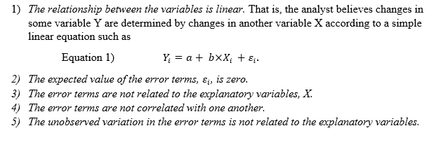
The simplest regression analysis is called ordinary least squares (OLS) because it determines the parameters of an estimated linear equation relating the variables by minimizing the sum of the squared differences between the observed values of the dependent variable (salaries, ticket prices and stock returns in our examples) and the independent or explanatory variables (education and tenure, dummy variable for before and after the attempted collusion and jet fuel prices, and stock index returns in our examples). The difference between observed values and predicted values for different values of the explanatory variable are called error terms or residuals.
OLS requires the following five key assumptions to hold for the regression results to be valid.
Two kinds of data
Successful application of regression analysis must recognize potential problems with the data being analyzed to ensure that faulty inferences are not drawn from naive application of a valid technique to problematic data.
Data sets include observations on a list of variables. In our labor example the data set might contain 2016 salaries, level of formal education, years with current employer and years as a CPA for 5,000 individual CPAs in New York. Each individual CPA's set of values comprise an observation and our hypothetical dataset contains 5,000 such observations. This data set is a cross sectional data set because all the observations are taken at approximately the same point in time. The variation in this example data set is across individual CPAs.
Time series data on the other hand is a set of observations in which the variation in observations is across time. For example, an analyst might use OLS to determine whether the yields on Treasury bonds are related to mortgage interest rates using a dataset that contains observations on Treasury yields and benchmark mortgage interest rates at each month end for a 10-year period (120 observations). The variation in this dataset is across time from one month to the next and the data.1
Sunspots and GNP
There are pervasive challenges applying regression analysis to time series data. An analyst who is not knowledgeable about basic statistics could conclude that two completely unrelated series are closely related by failing to test for serial correlation. This problem is especially acute in time series data where time trends and other omitted variables are likely to cause time series to move together even when there is no independent relationship between the variables. Fortunately, there are ways of drawing valid inferences from times series data with regression analysis which can be found in almost any introductory econometrics textbooks and are well-known to any competent analyst.
Simplifying Plosser and Schwert's example, imagine accumulating the sunspots observed each year into a running total. Such a series would increase each year by the number of sunspots observed that year. GNP also increases over time. Regressing GNP on cumulative sunspots generates a high R-squared and a significant t-statistic on cumulative sunspots even though GNP and sunspots are obviously unrelated. The analyst could avoid a possible embarrassing mistake by noting the residuals are positively correlated as evidenced by the DW statistic and make the correct transformation of the GNP and sunspots variables. This is a famous example because the regression of levels on levels is so obviously wrong and because regressing first differences (annual changes in GNP and sunspots) demonstrates that GNP and sunspots are unrelated other than by virtue of both having a positive time trend.
As Granger and Newbold in 1974 and Plosser and Schwert in 1978 made clear, the issue raised by time series data is not whether the variables should be measured as levels or as changes in levels, i.e. first differences of levels, but whether the resulting error terms are uncorrelated or not. If the error terms are correlated some remedial measure such as first differencing the variables must be taken or else the conclusions drawn from the regression analysis are not valid.
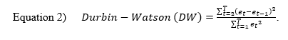
It is exceedingly hard to miss serial correlation in error terms since statistical packages automatically produce the Durbin-Watson (DW) statistic which tests for serial correlation of the error terms.2
The DW statistic ranges from 0 to 4; DW = 0 means the error terms are perfectly positively correlated, DW = 4 means the error terms are perfectly negatively correlated and DW = 2 means the error terms are uncorrelated.3 Statistical tables provide critical values for the DW statistic which would allow us to conclude at a given confidence level that the error terms are correlated, uncorrelated or of an indeterminate relationship.
Sunspots and GNP Revisited: Puerto Rico Municipal Bond Returns
Our recent research into Puerto Rico municipal bond returns provides an example of the potential for finding an unreliable relationship in time series data which can be avoided by paying attention to what the DW statistic tells us about serial correlation in the error terms.
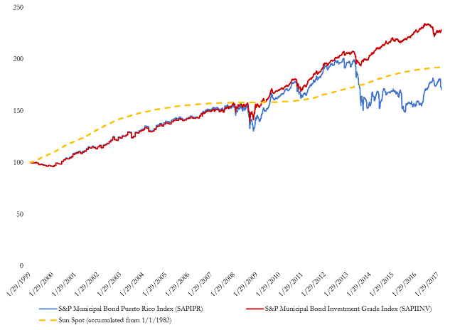
In Figure 1,We plot the S&P Puerto Rico Municipal Total Return Index (SAPIPR) and the S&P Investment Grade Municipal Total Return Index (SAPIINV) both set equal to 100 on January 29, 1999.We also plot the cumulative sunspots observed from January 1, 1982 normalized to equal 100 on January 29, 1999 when our total return data starts.4
As we expect from a fixed income total return index, there is a strong upward trend in both the Puerto Rico and USA series. There is a drop in both indexes in 2008, 2010 and 2013. Each time the drop in the Puerto Rico is larger than the drop in the USA series. The drop in Puerto Rico municipal bond prices in 2013 was especially dramatic and persistent.
Figure 1. S&P's Puerto Rico and Mainland Municipal Total Return Indexes
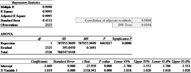
Figure 1 might tempt an unsophisticated analyst to run an OLS regression on these two total return index level data series from January 29, 1999 to December 31, 2007 to support a belief that Puerto Rico municipal bond returns are highly correlated with mainland municipal bond returns. The results of that regression run in Excel are reported in Tables 1.
Table 1. OLS Regression of Puerto Rico Total Return Index on USA Total Return Index
The R-squared statistic = 0.9995 and t-statistic = 2,159 on the explanatory variable are red flags that there is something wrong with this regression.5 As Granger and Newbold and Plosser and Schwert foretold, there is an extreme positive serial correlation problem with this regression. The correlation between adjacent residuals is 0.99 (should be near 0 on a scale from -1 to +1) and the DW statistic is 0.02 (should be near 2 on a scale from 0 to 4). Figure 2 plots the residuals on lagged residuals from the regression of S&P Puerto Rico Municipal Total Return Index level and the S&P Investment Grade Municipal Total Return Index level. This plot clearly shows the high correlation amongst adjacent error terms.
Figure 2. Residuals from Table 1 Regression Plotted Against Lagged Residuals
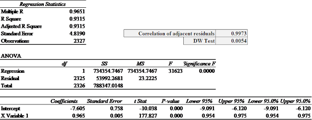
To see how silly it would be to defend the regression reported in Table 1 consider a regression of the Puerto Rico Municipal Bond Total Return on the Cumulative Sunspots variable plotted in Figure 1. Obviously Puerto Rico municipal bond returns are unrelated to sunspot activity yet the regression yields an R-Squared of 0.93 and a t-statistic on the Cumulative Sunspots of 177.8. See Table 2.
Table 2. OLS Regression of Puerto Rico Total Return Index on Cumulative Sunspots Since 1982
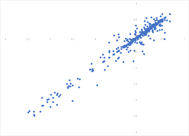
An analyst who accepts or defends the regression results reported in Table 1 would likely also accept and defend the nonsensical results in Table 2. The correlation coefficient for adjacent residuals from the regression in Table 2 is 0.997 and the DW statistic is 0.0054 demonstrating that the residuals are nearly perfectly positively correlated and the regression results therefore unreliable. Figure 3 is a residual plot for the Puerto Rico municipal bond total returns levels on cumulative sunspots. It looks very similar to Figure 2 because both regressions suffer from severe serial autocorrelation.
Figure 3. Residuals from Table 2 Regression Plotted Against Lagged Residuals
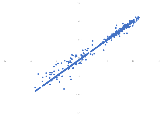
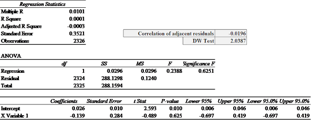
With near perfect positive serial autocorrelation like exhibited in Figure 2 and Figure 3 the standard fix is to run the regression on the first differences of the variables. The results of a regression of first differences in the Puerto Rico Municipal Bond Total Return Index and the Cumulative Sunspots are reported in Table 3. The R-Squared drops to 0 and the t-statistic on the Sunspots variable is not statistically significant at standard confidence levels. This is what we expect since Puerto Rico municipal bond returns cannot be related to sunspot activity. The correlation coefficient for adjacent residuals from the regression in Table 3 is -0.020 and the DW statistic is 2.039 demonstrating that the residuals are uncorrelated and the regression statistics therefore likely reliable.6
Table 3. OLS Regression of Puerto Rico Total Return Index on Daily Sunspots
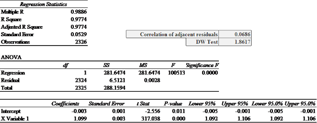
Returning to the more serious question of the relationship between the returns on Puerto Rican municipal bonds and the returns on mainland municipal bonds; as we saw in Table 1, the adjacent residuals are nearly perfectly correlated and so the careful analyst would run the regression on the first differences in the two total return index level variables. Table 4 reports the results of such a regression. The correlation coefficient of adjacent residuals is now 0.069 (instead of 0.99) and the DW statistic is 1.862 (instead of 0.02). The R-squared is still quite high and the statistic on the mainland variable is still implausibly high at 317 but the results in Table 4 make more sense than the results in Table 1.
Table 4. OLS Regression of Daily Changes in Puerto Rico Total Return Index on Daily Changes in USA Total Return Index
Take a Closer Look at the Data
There is a second major data problem that would cause the error terms to still be correlated. The index levels from 1999 to mid-2006 are only reported monthly.Our hypothetical hapless analyst has filled in all the missing days from 1999 to mid-2006 with the last value for both total return series and treated each day as having a new, independent observation instead of 20 identical observations.
Running OLS regressions on first differences of this "fake" data will still generate serially correlated errors since the error term every day but once a month during the period from January 1999 to August 2006 will equal the previous day's error term. The correlation coefficient and DW statistics reported above don't fully reflect the positive serial correlation because once a month there is a large reversal in error term. In fact, continuing to difference the variables a second time, a third time and so on as suggested by Plosser and Schwert won't fix this data problem. Even without looking at the DW statistic, the analyst would know by looking at the residuals from both the levels and differences regressions, the data from January 1999 to August 2006 is not daily data and can't be used as daily data.
There are other serious problems with analyzing this data and interpreting the results, but the lesson for today is simply: like any good undergraduate student, check the residuals for serial correlation.
_______________________________________
1 Panel data includes both cross-sectional variation and times series properties. For instance, a data set containing observations on salaries, level of formal education, years with current employer and years as a CPA for 5,000 CPAs over a 10 year period would be a panel data set. 2 A simple discussion of serial correlation can be found in any introductory econometrics textbook - even Econometrics for Dummies, Chapter 12. 3 Except for very small samples the DW statistic is equal to two times the difference between one and the correlation coefficient between adjacent error terms. That is DW=2×(1-ρ). If the error terms are perfectly positively correlated, ρ = 1 and DW = 0. If the error terms are perfectly negatively correlated, ρ = -1 and DW = 4. If the error terms are uncorrelated, ρ = 0 and DW = 2. 4 Source: WDC-SILSO, Royal Observatory of Belgium, Brussels. Downloaded at https://www.sidc.be/silso/datafiles. 5 T-statistics greater than 2.00 - not 2,000 - are usually considered to be statistically significant (more properly are statistically significant at the 5% confidence level). The R-squared statistic requires skeptical interpretation in every case and as reported in Table 1 at 0.999 is, literally, unbelievable. 6 This is too strong a statement since there could be other reasons why regression results might not be reliable but at least the error terms are uncorrelated which is a necessary assumption for the application of OLS to be valid.